> For the complete documentation index, see [llms.txt](https://gtae.gitbook.io/ae4610/llms.txt). Markdown versions of documentation pages are available by appending `.md` to page URLs; this page is available as [Markdown](https://gtae.gitbook.io/ae4610/archive/aero-lqr/2-dof-helicopter.md).

# A. System Identification

## Introduction

The Quanser Aero Experiment can be configured as a conventional dual-rotor helicopter, as shown in Figure 1. The front rotor that is horizontal to the ground predominantly affects the motion about the pitch axis while the back or tail rotor mainly affects the motion about the yaw axis (about the shaft).

![Fig. 1: Quanser Aero Experiment](https://1205030739-files.gitbook.io/~/files/v0/b/gitbook-legacy-files/o/assets%2F-MIedmBPpkGaOOtNl4mm%2F-MNoMImXG6dxo5hVNGFu%2F-MNoecZ-J58ZgtNeU11w%2Fimage.png?alt=media\&token=d184a89c-b1ba-4f0a-bf4b-d2a41dda311d)

The tail rotor in helicopters is also known as the anti-torque rotor because it is used to reduce the torque that the main rotor generates about the yaw. Without this, the helicopter would be difficult to stabilize about the yaw axis. The rotors on the Quanser Aero Experiment are the same size and equidistant from each other, the tail rotor also generates a torque about the pitch axis. As a result, both the front and back/tail rotors generate torques on each other.

## Background

### Pitch Stiffness

The Quanser 2D AERO is designed with its mass distribution well balanced from the front and back rotors such that its center of gravity is at the mid-point between the two rotors. However, a vertical offset of the cg location is included to result in pitch stiffness from the pendulum effect as depicted in the Figure.

<figure><img src="https://1205030739-files.gitbook.io/~/files/v0/b/gitbook-x-prod.appspot.com/o/spaces%2F-MIedmBPpkGaOOtNl4mm%2Fuploads%2FzUpoYbtt6o5aVBBhGcQT%2FScreenshot%202023-02-13%20104243.png?alt=media&amp;token=afadee50-bd2d-4364-9a5a-483f02af8f86" alt=""><figcaption><p>Figure: Pendulum effect creating pitch stiffness due to vertical offset of cg from pitch pivot.</p></figcaption></figure>

The system is in static equilibrium when it is horizontal and parallel to the ground with zero pitch angle. Any change in pitch angle $$\theta\_b$$ gives rise to a restoring moment from the pendulum effect given by restoring pitch moment due to pitch angle change = $$-M\_bgD\_m \sin(\theta\_b)\approx -M\_bgD\_m \theta\_b$$

### Equations of Motion

The free-body diagram of the Quanser Aero Experiment is illustrated in Figure 2.

![Fig. 2: Simple free-body diagram of Quanser Aero Experiment](https://1205030739-files.gitbook.io/~/files/v0/b/gitbook-legacy-files/o/assets%2F-MIedmBPpkGaOOtNl4mm%2F-MNoMImXG6dxo5hVNGFu%2F-MNooya_9MszcrIlGWEO%2Fimage.png?alt=media\&token=3f3f6577-ef6d-4cec-afbc-6bedc3aadc33)

The following conventions are used for the modeling:

* The helicopter is horizontal and parallel with the ground when the pitch angle is zero, i.e., $$\theta=0$$ .
* The pitch angle increases positively, $$\dot{\theta}(t)>0$$ , when the front rotor is moved upwards and the body rotates clockwise (CW) about the Y axis.
* The yaw angle increases positively, $$\dot{\psi}(t)>0$$ , when the body rotates counter-clockwise (CCW) about  &#x20;the Z axis.
* Pitch increases, $$\dot{\theta}>0$$ , when the front rotor voltage is positive $$V\_\theta>0$$ .
* Yaw increases, $$\dot{\psi}>0$$ , when the back (or tail) rotor voltage is positive, $$V\_{\psi}>0$$ .

When voltage is applied to the pitch motor, $$V\_\theta$$ , the speed of rotation results in a force, $$F\_\theta$$ that acts normal to the body at a distance $$r\_\theta$$ from the pitch axis. The rotation of the propeller generates a torque about the pitch rotor motor shaft which is in turn seen about the yaw axis. Thus, rotating the pitch propeller does not only cause motion about the pitch axis but also about the yaw axis. As described earlier, that is why conventional helicopters include a tail, or anti-torque, rotor to compensate for the torque generated about the yaw axis by the large, main rotor.

Similarly, the yaw motor causes a force $$F\_\psi$$ that acts on the body at a distance $$r\_\psi$$  from the yaw axis as well as a torque about the pitch axis.

The equations of motion can be approximated as:

&#x20;                                                                 $$J\_\theta\ddot{\theta}+D\_\theta\dot{\theta}+K\_\theta\theta=\tau\_\theta \tag{1}$$                                                                   &#x20;

$$J\_\psi\ddot{\psi}+ D\_\psi\dot{\psi}=\tau\_\psi \tag{2}$$​

where the torques acting on the pitch and yaw axes are &#x20;

&#x20;                                                                                      $$\tau\_\theta = K\_{\theta \theta} V\_{\theta} + K\_{\theta \psi} V\_{\psi} \tag{3}$$

$$\tau\_\psi = K\_{\psi \theta} V\_{\theta} + K\_{\psi \psi} V\_{\psi} \tag{4}$$​

The parameters used in the EOMs above are:

* $$J\_\theta$$ : the total moment of inertia about the pitch axis
* $$D\_\theta$$ : the damping about the pitch axis
* $$K\_\theta$$ : the stiffness about the pitch axis
* $$J\_{\psi}$$ : the total moment of inertia about the yaw axis
* $$D\_{\psi}$$ : the damping about the pitch axis
* $$K\_{\theta\theta}$$ : torque thrust gain from the pitch rotor
* $$K\_{\psi\psi}$$ : torque thrust gain from the yaw rotor
* $$K\_{\theta\psi}$$ : cross-torque thrust gain acting on the pitch from the yaw rotor
* $$K\_{\psi\theta}$$ : cross-torque thrust gain acting on the yaw from the pitch rotor
* $$V\_\theta$$ : voltage applied to the pitch rotor
* $$V\_\psi$$ : voltage applied to the yaw rotor motor

The total moment of inertia acting about the pitch and yaw axes are

&#x20;                                                                           $$J\_\theta=J\_{\rm body}+2J\_{\rm prop} \tag{5}$$                                                                 &#x20;

&#x20;                                                                     $$J\_\psi=J\_{\rm body}+2J\_{\rm prop}+J\_{\rm yoke} \tag{6}$$                                                      &#x20;

Expressing the rotor as a single-point mass, the inertia acting about the pitch or yaw axis from a single&#x20;rotor  is $$J\_{\rm prop}=m\_{\rm prop}r^2$$ . Modeling the helicopter body as a cylinder rotating about its center, the  inertia&#x20;is $$J=m\_{\rm body} \displaystyle  \frac{L^2\_{\rm body}}{12}$$. Finally, the forked yoke that rotates about the yaw axis can be approximated as&#x20;a cylinder rotating about its center as well and expressed as $$J\_{\rm yoke}=m\_{\rm yoke}\displaystyle \frac{r^2\_{yoke}}{2}$$. Evaluating the moment of inertia using the parameters listed in the Quanser Aero Experiment User Manual gives:

$$
J\_\theta=0.0219 \space \rm kg \cdot m^2
$$

$$
J\_\psi=0.0220\space \rm kg \cdot m^2
$$

### **First-Order Response**

The step response of a first-order transfer function

&#x20;                                                                            $$Y(s) = \displaystyle \frac{K}{\tau s+1}U(s) \tag{7}$$                                                                    &#x20;

where K is the DC or steady-state gain and τ is the time constant as illustrated in Figure 3. This is for a&#x20;system with $$K = 1$$ and $$\tau = 0.05$$.

To obtain the time constant from the response, find the time it takes to reach $$1-e^{-1}$$or 63% of its&#x20;final steady-state value:

$$y(t\_1)=y\_1=(1-e^{-1})(y\_{\rm ss}-y\_0) +y\_0 \tag{8a}$$

The time constant is $$\tau=t\_1-t\_{0 }$$, where $$t\_0$$ is the start time of the step and $$t\_1$$ is the time it takes to reach&#x20;63% of the final value, as illustrated in Figure 3.

![Fig. 3.a : First-order step response](https://1205030739-files.gitbook.io/~/files/v0/b/gitbook-legacy-files/o/assets%2F-MIedmBPpkGaOOtNl4mm%2F-MO8TAg0uFlzUjcVqCUP%2F-MO8ZM_nxDt9dWCWWd9-%2Fimage.png?alt=media\&token=bc39a812-8fc0-4c3c-99d5-d7b53d875579)

To find the time constant from first-order response from an impulse (or short step) as depicted in Figure 4, find the time it takes for the response to reach 37% of its initial pulse response.&#x20;

In this case we need to find&#x20;

$$y(t\_1)=y\_1=e^{-1}(y\_0 - y\_{ss})\tag{8b}$$

and the time constant is $$\tau=t\_1-t\_{0 }$$

<figure><img src="https://1205030739-files.gitbook.io/~/files/v0/b/gitbook-x-prod.appspot.com/o/spaces%2F-MIedmBPpkGaOOtNl4mm%2Fuploads%2FsSu6NDu3b8NdFEZPhq7D%2FScreenshot%202023-02-12%20221819.png?alt=media&amp;token=b1879177-6689-4fd1-bb38-8b3ed6e7d7c5" alt=""><figcaption><p>Figure 3.b: First-order impulse decaying response</p></figcaption></figure>

### Second-Order Response

The free-oscillatory equation of motion of a second-order system is described by

&#x20;                                                                      $$J\ddot{\alpha}+D\dot{\alpha}+K\alpha =0 \tag{9}$$                                                    &#x20;

is shown in Figure 4. Assuming the initial conditions $$\alpha(0-)=\alpha\_0$$, the Laplace transform of Equation (9)&#x20;is                    $$\alpha(s)=\displaystyle{\frac{\alpha\_0/J}{s^2+D/Js+K/J}}   \tag{10}$$                                                            &#x20;

The prototype second-order equation is defined

$$s^2+2\zeta\omega\_ns+\omega\_n^2 \tag{11}$$    &#x20;

where $$\zeta$$ is the damping ratio and $$\omega\_n$$ is the natural frequency. Equating the characteristic equation in&#x20;Equation (10) to this gives

$$\omega\_n^2=\displaystyle\frac{K}{J}\tag{12}$$​

$$2\zeta\omega\_n=\displaystyle\frac{D}{J} \tag{13}$$

#### Finding the Natural Frequency

The period of the oscillations in a system response can be found using the equation

&#x20;                                                                                $$T\_{\rm osc}=\displaystyle\frac{t\_n-t\_1}{n-1} \tag{14}$$                                                                           &#x20;

where $$t\_n$$ is the time of the $$n^{th}$$ oscillation, $$t\_1$$ is the time of the first peak, and $$n$$ is the number of&#x20;oscillations considered. From this, the damped natural frequency (in radians per second) is

&#x20;                                                                                 $$\omega\_d=\displaystyle \frac{2\pi}{T\_{\rm osc}} \tag{15}$$                                                                             &#x20;

and the undamped natural frequency is

&#x20;                                                                             $$\omega\_n=\displaystyle\frac{\omega\_d}{\sqrt{1-\zeta^2}} \tag{16}$$                                                                           &#x20;

#### Finding the Damping Ratio&#xD;

The damping ratio of a second-order system can be found from its response. For a typical second-order&#x20;underdamped system, the subsidence ratio (i.e. decrement ratio) is defined as

&#x20;                                                                            $$\delta = \displaystyle\frac{1}{n-1}\ln\frac{O\_1}{O\_n} \tag{17}$$&#x20;

![Fig. 4: Free Oscillation Response](https://1205030739-files.gitbook.io/~/files/v0/b/gitbook-legacy-files/o/assets%2F-MIedmBPpkGaOOtNl4mm%2F-MO8TAg0uFlzUjcVqCUP%2F-MO8i_-_o1XPQpRvSpBR%2Fimage.png?alt=media\&token=3d02c8bd-5bb1-4bec-abe1-034e0f71b89a)

where $$O\_1$$ is the peak of the first oscillation and $$O\_n$$ is the peak of the $$n^{th}$$ oscillation. Note that $$O\_1$$ > $$O\_n$$ ,&#x20;as this is a decaying response. The damping ratio can then be found using

&#x20;                                                                              $$\zeta= \displaystyle\frac{\delta}{\sqrt{4\pi^2+\delta^2}} \tag{18}$$                                                                          &#x20;

### Estimating the Viscous Damping Coefficients&#xD;

The viscous damping coefficients acting about the pitch and yaw axes, $$D\_\theta$$ and $$D\_\psi$$ in Equation (1)&#x20;and Equation (2), can be found from the free-oscillation response. The free-oscillation response about the&#x20;pitch and about the yaw are different, however.&#x20;

**Pitch Axis:** By locking the yaw axis (using the Allen key supplied), this allows us to focus on the&#x20;1 DOF pitch-only system. Apply a short step voltage to mimic an impulse and get the free-oscillation&#x20;response of the pitch. Remark that the impulse response is second-order free-oscillation response. The&#x20;resulting 1 DOF pitch-only equations of motion is

&#x20;                                                               $$J\_\theta\ddot{\theta}+D\_\theta\dot{\theta}+K\_\theta\theta=0 \tag{19}$$                                                               &#x20;

Taking its Laplace transform gives

&#x20;                       $$J\_\theta\left(\Theta(s)s^2-\theta(0^-)-\dot{\theta}(0^-)\right)+D\_\theta\left(\Theta(s)-\theta(0^-)\right)+K\_\theta\Theta(s)=0 \tag{20}$$                  &#x20;

Assuming the initial velocity is zero, $$\dot{\theta}(0^-)=0$$, and solving for position we get

&#x20;                                          $$\Theta(s)=\displaystyle\frac{J\_\theta}{J\_\theta s^2+D\_\theta s+K\_\theta}\theta(0^-)=\frac{J\_\theta D\_\theta}{s^2+D\_\theta/J\_\theta +K\_\theta/J\_\theta}\theta(0^-) \tag{21}$$                                   &#x20;

The pitch free-oscillation transfer function matches the prototype second-order transfer function in Equation (10) Based on the measured damping ratio and natural frequency of the response, the friction (or&#x20;stiffness) of the system is

&#x20;                                                                             $$K\_\theta=J\_\theta\omega\_n^2 \tag{22}$$                                                                             &#x20;

and the viscous damping is

&#x20;                                                                            $$D\_\theta=2\zeta\omega\_nJ\_\theta \tag{23}$$                                                                         &#x20;

**Yaw Axis:** The 1 DOF yaw-only equations of motion is

$$J\_\psi\ddot\psi+D\_\psi\dot\psi=0 \tag{24}$$

In terms of angular rate, the equation becomes

&#x20;                                                                     $$J\_\psi\dot\omega\_\psi(t)+D\_\psi\omega\_\psi(t)=0 \tag{25}$$                                                          &#x20;

where $$\omega\_\psi(t)=\dot{\psi}(t)$$ . Taking its Laplace transform

&#x20;                                                        $$J\_\theta(\Omega\_\psi(s)s-\omega\_\psi(0^-))+D\_\psi\Omega\_\psi(s)=0 \tag{26}$$                                          &#x20;

and solving for the speed we get

$$\Omega\_\psi(s)=\displaystyle \frac{J\_\psi}{J\_\psi s+D\_\psi}\omega\_\psi(0^-)=\frac{J\_\psi/D\_\psi}{J\_\psi/D\_\psi s+1}\omega\_\psi(0^-) \tag{27}$$

&#x20;The yaw free-oscillation transfer function matches the prototype first-order transfer function in Equation (7). Based on the measured time constant of the response, its damping can be found with

&#x20;                                                                                 $$D\_\psi=\displaystyle\frac{J\_\psi}{\tau} \tag{28}$$                                                                              &#x20;

### Estimating the Thrust Parameters&#xD;

By locking the yaw axis, this allows us to focus on the 1 DOF pitch-only system, i.e., eliminating any&#x20;motion introduced in the yaw axis when applying a voltage to the pitch rotor. The equations of motion&#x20;for the 1-DOF actuated system is

&#x20;                                                               $$J\_\theta\ddot\theta+D\_\theta\dot\theta+K\_\theta\theta=K\_{\theta\theta}V\_\theta \tag{29}$$                                                          &#x20;

Solving for the thrust gain we get

&#x20;                                                                         $$K\_{\theta\theta}=\displaystyle \frac{J\_\theta\ddot\theta+D\_\theta\dot\theta+K\_\theta\theta}{V\_\theta} \tag{30}$$                                                                 &#x20;

Remark that this is the thrust torque gain parameter. To force thrust gain would be $$K\_{\theta\theta}/r\_p$$, where $$r\_p$$is&#x20;the distance between the helicopter pivot and the center of the pitch rotor.&#x20;Similarly, to find the thrust gain acting on the yaw axis only system, lock the pitch axis, and apply a&#x20;voltage to the tail rotor. This system is represented by

&#x20;                                                                       $$J\_\psi\ddot\psi+D\_\psi\dot\psi=K\_{\psi\psi}V\_\psi \tag{31}$$                                                           &#x20;

or,

&#x20;                                                                      $$J\_\psi\dot\omega\_\psi+D\_\psi\omega\_\psi=K\_{\psi\psi}V\_\psi \tag{32}$$                                                        &#x20;

where $$\omega\_\psi=\dot\psi$$ is the angular rate of the yaw axis. The yaw torque thrust gain is

&#x20;                                                                             $$K\_{\psi\psi}=\displaystyle\frac{J\_\psi\dot\omega\_\psi+D\_\psi\omega\_\psi}{V\_\psi} \tag{33}$$                                                               &#x20;

The cross-torque thrust parameters, $$K\_{\theta\psi}$$and $$K\_{\psi\theta}$$in Equation (3) and (4), represent the coupling between the&#x20;axes. To find the cross-torque acting on the pitch axis from a torque applied to the tail rotor, unlock both&#x20;pitch and yaw axes such that it is free to move in 2 DOF, apply a voltage to the tail rotor, and examine&#x20;the response of the pitch. The equations representing these dynamics when $$V\_\theta=0$$ , are

&#x20;                                                                     $$J\_\theta\ddot\theta+D\_\theta\dot\theta+K\_\theta\theta=K\_{\theta\psi}V\_\psi \tag{34}$$                                                   &#x20;

Putting this in terms of angular rate, $$\omega\_p=\dot\theta$$, and solving for the gain we get

&#x20;                                                                                $$K\_{\theta\psi}=\displaystyle\frac{J\_\theta\dot\omega\_\theta+D\_\theta\omega\_{\theta}}{V\_\psi} \tag{35}$$                                                               &#x20;

Similarly, to identify the cross-torque gain parameter that is generated about the yaw axis from a pitch&#x20;torque (i.e. voltage applied to the front rotor), we have the equation

&#x20;                                                                          $$J\_\psi\ddot\psi+D\_\psi\dot\psi=K\_{\psi\theta}V\_\theta \tag{36}$$                                                          &#x20;

and the gain can be found using

&#x20;                                                                             $$K\_{\psi\theta}=\displaystyle\frac{J\_{\psi}\dot\omega\_\psi+D\_\psi\omega\_{\psi}}{V\_\theta} \tag{37}$$                                                             &#x20;

## A. System Identification

### Experimental Steps for Finding System Parameters

First download the zip file below and extract it in the desktop:

{% file src="/files/ujeep9YMvwh1zmrKc1Km" %}

#### 1. Finding Pitch Damping, $$D\_{\theta}$$

1\) Lock the yaw axis to enable motions about the pitch axis only. (place the allen key to lock yaw axis and make sure that the pitch axis is free to rotate, loosen two screws)

2\) Open the *q\_aero\_free\_osc\_response\_pitch SIMULINK file.*

3\) Impulse of -20V for 1.5s.

4\) Select simulation time 30 sec.

5\) To build the model, click the down arrow on **Monitor & Tune** under the Hardware tab and then click **Build** **for monitoring** ![](https://1205030739-files.gitbook.io/~/files/v0/b/gitbook-x-prod.appspot.com/o/spaces%2F-MIedmBPpkGaOOtNl4mm%2Fuploads%2FCq5iMDIRj3JN7fcFsx2w%2Fimage.png?alt=media\&token=6ffaf234-92d6-4de2-be27-7a37a4fe9dcc). This generates the controller code.

6\) Click **Connect** <img src="https://1205030739-files.gitbook.io/~/files/v0/b/gitbook-x-prod.appspot.com/o/spaces%2F-MIedmBPpkGaOOtNl4mm%2Fuploads%2F1VD5IqnbVgR6hbi4YOei%2Fimage.png?alt=media&amp;token=02e68127-9611-4c74-b03f-b7cac5c04a34" alt="" data-size="line"> button under **Monitor & Tune** and then run SIMULINK by clicking **Start** <img src="https://1205030739-files.gitbook.io/~/files/v0/b/gitbook-x-prod.appspot.com/o/spaces%2F-MIedmBPpkGaOOtNl4mm%2Fuploads%2F5kUOzUmpIz5Mob4x7xd1%2Fimage.png?alt=media&amp;token=60cb4298-b97c-4538-8240-2d44c2d721b0" alt="" data-size="line">.

7\) Copy *`aero_pitch_free_osc_rsp.mat`* to your folder. \
\
Data is saved in following order:\
1: Time (s) \
2: Pitch input (V) \
3: Pitch position (rad) \
4: Pitch speed (rad/s) \
5: Pitch acceleration (rad/s^2)

8\) Close the SIMULINK model. DO NOT SAVE THE CHANGE

![Fig. 5: Sample free-oscillation response about pitch](https://1205030739-files.gitbook.io/~/files/v0/b/gitbook-x-prod.appspot.com/o/spaces%2F-MIedmBPpkGaOOtNl4mm%2Fuploads%2FHuYKrRtJc2Qn4hbMSkM6%2F2_6.png?alt=media\&token=53aa5232-0e14-40db-a6c2-6e181b8150a6)

#### 2. Finding Pitch thrust gain, $$K\_{\theta\theta}$$&#x20;

1\) Open the *q\_aero\_step\_response\_pitch SIMULINK file.*

2\) Select a step voltage 24V, (amplitude to 24)

3\) Select simulation time 30 sec.

4\) To build the model, click the down arrow on **Monitor & Tune** under the Hardware tab and then click **Build** **for monitoring** ![](https://1205030739-files.gitbook.io/~/files/v0/b/gitbook-x-prod.appspot.com/o/spaces%2F-MIedmBPpkGaOOtNl4mm%2Fuploads%2FCq5iMDIRj3JN7fcFsx2w%2Fimage.png?alt=media\&token=6ffaf234-92d6-4de2-be27-7a37a4fe9dcc). This generates the controller code.

5\) Click **Connect** <img src="https://1205030739-files.gitbook.io/~/files/v0/b/gitbook-x-prod.appspot.com/o/spaces%2F-MIedmBPpkGaOOtNl4mm%2Fuploads%2F1VD5IqnbVgR6hbi4YOei%2Fimage.png?alt=media&amp;token=02e68127-9611-4c74-b03f-b7cac5c04a34" alt="" data-size="line"> button under **Monitor & Tune** and then run SIMULINK by clicking **Start** <img src="https://1205030739-files.gitbook.io/~/files/v0/b/gitbook-x-prod.appspot.com/o/spaces%2F-MIedmBPpkGaOOtNl4mm%2Fuploads%2F5kUOzUmpIz5Mob4x7xd1%2Fimage.png?alt=media&amp;token=60cb4298-b97c-4538-8240-2d44c2d721b0" alt="" data-size="line">.

6\) Copy *`aero_pitch_step_rsp.mat`* to your folder.\
\
Data is saved in following order: \
1: Time \
2: Pitch input (V) \
3: Pitch position (rad) \
4: Pitch Speed (rad/s)

7\) Close the SIMULINK model. DO NOT SAVE THE CHANGE.

<figure><img src="https://1205030739-files.gitbook.io/~/files/v0/b/gitbook-x-prod.appspot.com/o/spaces%2F-MIedmBPpkGaOOtNl4mm%2Fuploads%2FlFWnenNjvpqNasrVRLkw%2Funtitled.jpg?alt=media&amp;token=67e5ada2-75a9-4e04-90a6-722b37675d85" alt=""><figcaption><p>Fig. 6: Sample Pitch Step Response</p></figcaption></figure>

#### 3. Finding Yaw Damping , $$D\_{\psi}$$

1\) Unlock the yaw axis

2\) Lock the pitch axis

3\) Open the *q\_aero\_free\_osc\_response\_yaw SIMULINK file.*

4\) Apply an impulse of 20V to the tail rotor for 1s.

5\) Select simulation time 10 sec.

6\) To build the model, click the down arrow on **Monitor & Tune** under the Hardware tab and then click **Build** **for monitoring** ![](https://1205030739-files.gitbook.io/~/files/v0/b/gitbook-x-prod.appspot.com/o/spaces%2F-MIedmBPpkGaOOtNl4mm%2Fuploads%2FCq5iMDIRj3JN7fcFsx2w%2Fimage.png?alt=media\&token=6ffaf234-92d6-4de2-be27-7a37a4fe9dcc). This generates the controller code.

7\) Click **Connect** <img src="https://1205030739-files.gitbook.io/~/files/v0/b/gitbook-x-prod.appspot.com/o/spaces%2F-MIedmBPpkGaOOtNl4mm%2Fuploads%2F1VD5IqnbVgR6hbi4YOei%2Fimage.png?alt=media&amp;token=02e68127-9611-4c74-b03f-b7cac5c04a34" alt="" data-size="line"> button under **Monitor & Tune** and then run SIMULINK by clicking **Start** <img src="https://1205030739-files.gitbook.io/~/files/v0/b/gitbook-x-prod.appspot.com/o/spaces%2F-MIedmBPpkGaOOtNl4mm%2Fuploads%2F5kUOzUmpIz5Mob4x7xd1%2Fimage.png?alt=media&amp;token=60cb4298-b97c-4538-8240-2d44c2d721b0" alt="" data-size="line">.

8\) Copy *`aero_yaw_free_osc_rsp.mat`* to your folder\
\
Data is saved in following order: \
1: Time (s) \
2: Yaw input (V) \
3: Yaw position (rad) \
4: Yaw speed (rad/s) \
5: Yaw acceleration (rad/s^2)\\

9\) Close the SIMULINK model. DO NOT SAVE THE CHANGE.

<figure><img src="https://1205030739-files.gitbook.io/~/files/v0/b/gitbook-x-prod.appspot.com/o/spaces%2F-MIedmBPpkGaOOtNl4mm%2Fuploads%2FM4Bj4xQhbkDf81wZP4Ja%2F2_7.png?alt=media&amp;token=b5922435-bbdb-4533-bbaf-b98b92aae3e2" alt=""><figcaption><p>Fig. 7: Sample free response about yaw</p></figcaption></figure>

#### 4. Finding Yaw thrust gain, $$K\_{\psi\psi}$$&#x20;

1\) Open the *q\_aero\_step\_response\_yaw SIMULINK file.*

2\) Select a step voltage 15V

3\) Select simulation time 60 sec.

4\) To build the model, click the down arrow on **Monitor & Tune** under the Hardware tab and then click **Build** **for monitoring** ![](https://1205030739-files.gitbook.io/~/files/v0/b/gitbook-x-prod.appspot.com/o/spaces%2F-MIedmBPpkGaOOtNl4mm%2Fuploads%2FCq5iMDIRj3JN7fcFsx2w%2Fimage.png?alt=media\&token=6ffaf234-92d6-4de2-be27-7a37a4fe9dcc). This generates the controller code.

5\) Click **Connect** <img src="https://1205030739-files.gitbook.io/~/files/v0/b/gitbook-x-prod.appspot.com/o/spaces%2F-MIedmBPpkGaOOtNl4mm%2Fuploads%2F1VD5IqnbVgR6hbi4YOei%2Fimage.png?alt=media&amp;token=02e68127-9611-4c74-b03f-b7cac5c04a34" alt="" data-size="line"> button under **Monitor & Tune** and then run SIMULINK by clicking **Start** <img src="https://1205030739-files.gitbook.io/~/files/v0/b/gitbook-x-prod.appspot.com/o/spaces%2F-MIedmBPpkGaOOtNl4mm%2Fuploads%2F5kUOzUmpIz5Mob4x7xd1%2Fimage.png?alt=media&amp;token=60cb4298-b97c-4538-8240-2d44c2d721b0" alt="" data-size="line">.

6\) Copy *`aero_yaw_step_rsp.mat`* to your folder\
\
Data is saved in following order: \
1: Time \
2: Yaw input (V) \
3: Yaw position (rad) \
4: Yaw Speed (rad/s)\\

7\) Close the SIMULINK model. DO NOT SAVE THE CHANGE.

<figure><img src="https://1205030739-files.gitbook.io/~/files/v0/b/gitbook-x-prod.appspot.com/o/spaces%2F-MIedmBPpkGaOOtNl4mm%2Fuploads%2FqHhtJb27tj1Q9EDgSwKS%2F2_10.png?alt=media&amp;token=90e565ee-82fe-42d9-a46f-bfd3d40bb42e" alt=""><figcaption><p>Fig. 8: Sample yaw Step Response</p></figcaption></figure>

#### 5. Identifying the cross-torque gain parameter $$K\_{\theta\psi}$$&#xD;

1\) Unlock both the pitch and yaw axes to enable the full 2 DOF motion.

2\) Open the *q\_aero\_step\_response\_pitch\_from\_yaw SIMULINK file.*

3\) Select yaw step voltage to 12V and pitch to 0V.

4\) Select simulation time 40 sec.

5\) To build the model, click the down arrow on **Monitor & Tune** under the Hardware tab and then click **Build** **for monitoring** ![](https://1205030739-files.gitbook.io/~/files/v0/b/gitbook-x-prod.appspot.com/o/spaces%2F-MIedmBPpkGaOOtNl4mm%2Fuploads%2FCq5iMDIRj3JN7fcFsx2w%2Fimage.png?alt=media\&token=6ffaf234-92d6-4de2-be27-7a37a4fe9dcc). This generates the controller code.

6\) Click **Connect** <img src="https://1205030739-files.gitbook.io/~/files/v0/b/gitbook-x-prod.appspot.com/o/spaces%2F-MIedmBPpkGaOOtNl4mm%2Fuploads%2F1VD5IqnbVgR6hbi4YOei%2Fimage.png?alt=media&amp;token=02e68127-9611-4c74-b03f-b7cac5c04a34" alt="" data-size="line"> button under **Monitor & Tune** and then run SIMULINK by clicking **Start** <img src="https://1205030739-files.gitbook.io/~/files/v0/b/gitbook-x-prod.appspot.com/o/spaces%2F-MIedmBPpkGaOOtNl4mm%2Fuploads%2F5kUOzUmpIz5Mob4x7xd1%2Fimage.png?alt=media&amp;token=60cb4298-b97c-4538-8240-2d44c2d721b0" alt="" data-size="line">.

{% hint style="info" %}
A pitch up motion must be seen due to torque from the tail rotor.
{% endhint %}

7\) Copy *`aero_pitch_from_yaw_step_rsp.mat`* to your folder\
\
Data is saved in following order: \
1: Time (s)\
2: Yaw input (V) \
3: Pitch Position (rad) \
4: Pitch Speed (rad/s)\\

8\) Close the SIMULINK model. DO NOT SAVE THE CHANGE.
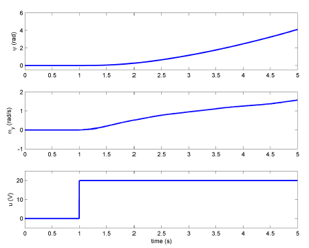
<figure><img src="https://1205030739-files.gitbook.io/~/files/v0/b/gitbook-x-prod.appspot.com/o/spaces%2F-MIedmBPpkGaOOtNl4mm%2Fuploads%2F2xEobFfm6PuurZG6zteV%2F2_11.png?alt=media&amp;token=8126d063-e815-4d30-aa74-92a29b91b90f" alt=""><figcaption><p>Fig. 9: Sample Pitch Step Response from Yaw Voltage</p></figcaption></figure>

#### 6. Identifying the cross-torque gain parameter $$K\_{\psi\theta}$$&#xD;

1\) Open the *q\_aero\_step\_response\_yaw\_from\_pitch SIMULINK file.*

2\) Select pitch step voltage to 12V and yaw to 0V.

3\) Select simulation time 40 sec.

4\) To build the model, click the down arrow on **Monitor & Tune** under the Hardware tab and then click **Build** **for monitoring** ![](https://1205030739-files.gitbook.io/~/files/v0/b/gitbook-x-prod.appspot.com/o/spaces%2F-MIedmBPpkGaOOtNl4mm%2Fuploads%2FCq5iMDIRj3JN7fcFsx2w%2Fimage.png?alt=media\&token=6ffaf234-92d6-4de2-be27-7a37a4fe9dcc). This generates the controller code.

5\) Click **Connect** <img src="https://1205030739-files.gitbook.io/~/files/v0/b/gitbook-x-prod.appspot.com/o/spaces%2F-MIedmBPpkGaOOtNl4mm%2Fuploads%2F1VD5IqnbVgR6hbi4YOei%2Fimage.png?alt=media&amp;token=02e68127-9611-4c74-b03f-b7cac5c04a34" alt="" data-size="line"> button under **Monitor & Tune** and then run SIMULINK by clicking **Start** <img src="https://1205030739-files.gitbook.io/~/files/v0/b/gitbook-x-prod.appspot.com/o/spaces%2F-MIedmBPpkGaOOtNl4mm%2Fuploads%2F5kUOzUmpIz5Mob4x7xd1%2Fimage.png?alt=media&amp;token=60cb4298-b97c-4538-8240-2d44c2d721b0" alt="" data-size="line">.

{% hint style="info" %}
A yaw motion must be seen due to torque from front motor.
{% endhint %}

6\) Copy *`aero_yaw_from_pitch_step_rsp.mat`* to your folder\
\
Data is saved in following order: \
1: Time (s) \
2: Pitch input (V) \
3: Yaw Position (rad) \
4: Yaw Speed (rad/s)

7\) Close the SIMULINK model. DO NOT SAVE THE CHANGE.

![Fig. 10: Sample Yaw Step Response from Pitch Voltage](https://1205030739-files.gitbook.io/~/files/v0/b/gitbook-x-prod.appspot.com/o/spaces%2F-MIedmBPpkGaOOtNl4mm%2Fuploads%2FEs5kFgeyyL97kRmTANVD%2F2_12.png?alt=media\&token=1139d008-8727-4edf-8c2f-41dbaee6a7b9)

### Analysis&#x20;

1. Find the **natural frequency** and **damping ratio** from the impulse response of the **pitch axis** (HINT: first find the peaks and use equation 16, 17, and 18). Then find the **stiffness** and **viscous damping coefficient** about the **pitch axis** (Hint: equation 22,23).

2. Find the **time constant** from the **yaw pulse** response and obtain the **damping** $$D\_\psi$$. Use First-order impulse decaying response. To find the time constant, examine the decaying response that starts at an initial maximum speed and settle down to 0 rad/s (use equation 8b). If data obtained does not fully shows the 37% of $$y\_0$$ try estimate the value by curve fitting.<br>

3. Find the **thrust** and **cross-torque thrust gain** parameters $$K\_{\theta\theta}, K\_{\psi\psi}, K\_{\theta\psi}, K\_{\psi\theta}$$ \
   \
   $$K\_{\theta\theta} = \displaystyle\frac{\theta\_{ss}K\_{\theta}}{V\_\theta} \tag{38}$$\\

$$K\_{\psi\psi}=\displaystyle\frac{J\_\psi\dot\omega\_\psi+D\_\psi\omega\_\psi}{V\_\psi} \tag{33}$$

$$K\_{\theta\psi} = \displaystyle\frac{\theta\_{ss}K\_{\theta}}{V\_\psi}  \tag{39}$$

$$K\_{\psi\theta}=\displaystyle\frac{J\_\psi\dot\omega\_\psi+D\_\psi\omega\_\psi}{V\_\theta} \tag{33}$$

Hint: $$\dot{\omega\_\psi}$$can be obtained by using MATLAB function diff(psi\_dot)/h, where h is sampling time. Compute $$K\_{\psi\psi}$$ by using the psi\_ddot(start:end), psi\_dot(start:end) and V\_psi(start:end) from start to end of step input. Do matrix division and you should get one $$K\_{\psi\psi}$$ value.\ <br>
