C. Controller Implementation (Week 2)

Objective

In this section, the gyroscopic control developed in Part B is implemented on the actual hardware. The goal is to see if the gyro module can maintain its heading $(\psi)$ when a disturbance is added by the user, i.e., the base plate is rotated.

The controller will also enable the gyroscope to track a small step, large step and ramp-input commands.

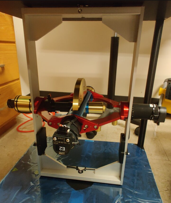
The q_3dgyro_reaction_torque_m2021.slx diagram shown in Figure 8 is used to implement the controller on the Quanser Gyroscope system. The 3 DOF Gyroscope system shown in Figure 9 contains the Quanser blocks that interface with their hardware.

Figure 8. q_3dgyro_reaction_torque_m2021 Simulink diagram

Figure 9. 3 DOF Gyroscope Simulink subsystem

3KB

gyro_sim_data.mlx

59KB

q_3dgyro_reaction_torque_m2021.slx

Part 1: Heading-hold experiment

1. Orient the gyroscope discs as shown:

Figure 10. Gyroscope orientation for heading-hold, facing side opposite wires

2. Make sure the pitch axis/red gimbal is locked.

3. Make sure the gray frame and blue gimbal ($\psi$ and $\phi$ respectively) are unlocked.

Note: Show your setup to your TA before proceeding. This will be the default orientation for all subsequent experiments.

4. Turn on the amplifier (big box) and verify the DAQ (small box) is connected to a power source. In previous experiments the smaller DAQ boards could be powered by the computer USB connection, but this is no longer the case.

5. Run gyro_sim_data.mlx script in MATLAB 2021 (not 2019) to initialize values.

6. Open q_3dgyro_reaction_torque.m2021.slx in MATLAB 2021 as well.

7. Set the $k_p, \,\, k_d \,\,$and $k_v$ values to those found in Week 1 Part B.

8. Set the Psi_Ref to 0. This will make the controller hold the 0-degree heading.

9. Set Hardware > Stop Time to 20 seconds.

10. Open all three scopes (Disc Rate, phi, psi) in a separate window.

11. When ready with the provided ruler, press Monitor & Tune (no need to build).

12. Watch the Disc Rate scope. When the angular velocity of the wheel reaches its maximum of ~78 rad/s, push the gray axis using the ruler at different angles/locations. Observe the behavior of the setup and notice the resistance to your disturbance by the gray axis, even though it is stationary.

IMPORTANT: After the experiment stops, use the provided towel to slowly stop the disc from spinning. Be careful since touching the disc while it is rotating may cause injury.

13. Check the saved data for disk rate, phi and psi, labelled as omega, phi, psi respectively. These are automatically saved as .mat files in your working directory. Rename them with "part1_" as the prefix, followed by the variable name. The data is saved as follows:

• The variable omega has the rows saving time, commanded speed, and actual speed respectively.

• The variable phi saves time, phi response, and phi gimbal current respectively.

• The variable psi saves time, reference psi angle, and psi response respectively.

Part 2: Small step response

1. Make sure the disc is fully stopped from the previous experiment.

2. Orient the gyroscope as shown in Figure 10.

3. Set simulation Stop Time to 20 seconds.

4. Set Psi_Ref to 0, apply the change, but keep the window open.

5. Open all three scopes in a separate monitor.

6. Click Monitor & Tune, and watch the Disc Rate scope.

7. When disc rate reaches its maximum, change Psi_Ref (deg) gain to 10 degrees.

8. Observe the gyroscope tracking the desired heading command.

IMPORTANT: After the experiment stops, use the provided towel to slowly stop the disc from spinning. Be careful since touching the disc while it is rotating may cause injury.

9. Refer to Part 1 Step 13 for the saved data format. Rename them with "part2_" as prefix, followed by the variable names as shown in Part 1 step 13.

Part 3: Large step response

1. Make sure the disc is fully stopped from the previous experiment.

2. Orient the gyroscope as shown in Figure 10.

3. Set simulation Stop Time to 20 seconds.

4. Set Psi_Ref (deg) gain to 0, apply the change, but keep the window open.

5. Open all three scopes in a separate monitor.

6. Click Monitor & Tune, and watch the Disc Rate scope.

7. When disc rate reaches its maximum, change Psi_Ref (deg) gain to 40 degrees.

8. Observe the gyroscope tracking the desired heading command.

IMPORTANT: After the experiment stops, use the provided towel to slowly stop the disc from spinning. Be careful since touching the disc while it is rotating may cause injury.

9. Refer to Part 1 Step 13 for the saved data format. Rename them with "part3_" as the prefix, followed by the variable names shown in Part 1 step 13.

Part 4: Ramp input response

While the step response is useful for system characterization, it is seldom used for an actual in-service trajectory because it is excessively harsh (high acceleration and jerk, which is the rate of change of acceleration). A more common trajectory used for tracking applications is a ramp.

1. Make sure the disc is fully stopped from the previous experiment.

2. Orient the gyroscope as shown in Figure 10.

3. Set simulation Stop Time to 20 seconds.

4. Open the Signal Generator block, and select the “sawtooth” waveform

5. Set Psi_Ref (deg) gain to 0, apply the change, but keep the window open.

6. Open all three scopes in a separate monitor.

7. Click Monitor & Tune, and watch the Disc Rate scope.

8. When disc rate reaches its maximum, change Psi_Ref (deg) gain to 20 degrees.

9. Observe the gyroscope tracking the desired heading command.

IMPORTANT: After the experiment stops, use the provided towel to slowly stop the disc from spinning. Be careful since touching the disc while it is rotating may cause injury.

10. Refer to Part 1 Step 13 for the saved data format. Rename them with "part4_" as the prefix, followed by the variable names shown in Part 1 step 13.

Results for Report

Note: Some results require simulation response. This would require running a simulation using your SIMULINK model from Part B Control Design using the same $k_p$, $k_d$ and $k_v$ gain values evaluated in Part C Controller Implementation. The command input will be identical to either the square wave signal or triangle signal implemented during the experiment. The simulation command input should be identical to experimental input.

1. Briefly describe the controller implementation experiments.

Part 1: Heading hold

1. Plot $\psi$ commanded and $\psi$ response plots on the same axes.

2. Plot $\phi$ response.

3. Plot motor 2 current ($\phi$ gimbal control current).

4. Explain the behavior of the gray axis as you disturb it.

Part 2: Small step input

1. Plot $\psi$ commanded, $\psi$ simulated, and $\psi$ experimental plots on the same axes.

2. Plot $\phi$ simulated and $\phi$ experimental responses on the same axes.

3. Plot motor 2 current simulated and experimental responses on the same axes.

4. Explain any differences between simulated and experimental responses.

Part 3: Large step input

1. Plot $\psi$ commanded and $\psi$ response plots on the same axes.

2. Plot $\phi$ response.

3. Plot motor 2 current.

Part 4: Ramp input

1. Plot $\psi$ commanded and $\psi$ response plots on the same axes.

2. Plot $\phi$ response.

3. Plot motor 2 current.

Questions for Report

1. There is some drift in the $\phi$ response overtime in all experiments. Despite this, the control is still able to maintain the desired yaw position. Explain using conservation of angular momentum and control theory why this is the case.

2. Which axis of the setup is fixed to the spacecraft?

3. Using the gyroscopic principle, what changes would you make to the gyroscope system for measuring yaw rate of the spacecraft?